A trend in geostatistics could be a general tendency in the direction industry is taking, like toward automation. A trend in geostatistics is also a non-stationary or locally-varying mean in a regionalized variable, particularly for a continuous variable. We would denote such a trend as $\{E\{Z(\mathbf{u})\}=m(\mathbf{u}), \mathbf{u}\; in\; A\}$. This kind of trend is common and must be considered in probabilistic resource modeling; otherwise, high values are smeared into volumes they do not belong and low values dilute high valued volumes. Two questions arise: (1) how to model the trend? and (2) how to model with a trend?

Trends introduce challenges in workflows for probabilistic resource estimation. There are rarely enough data to enforce the large-scale trend-like features in simulated realizations; high and low values will overly influence locations where they do not belong. Trends also confound the correct histogram to reproduce; validating the simulated realizations becomes challenging. Conventional estimation with ordinary kriging is quite robust with respect to a trend. Simulation, however, depends more on the global stationary histogram. Explicit consideration of a trend in simulation is commonly required.

A continuous regionalized variable $\{Z(\mathbf{u}), \mathbf{u}\; in\; A\}$ is not intrinsically composed of a deterministic trend and stochastic residual; nevertheless, there are large scale volumes of higher and lower values within a nominally stationary domain. Dividing the domain into smaller domains that appear more stationary may be an option, but the number of data reduces and artificial discontinuities are introduced at domain boundaries. Maintaining reasonably large domains for modeling and explicitly considering a trend has proven useful in many case studies.

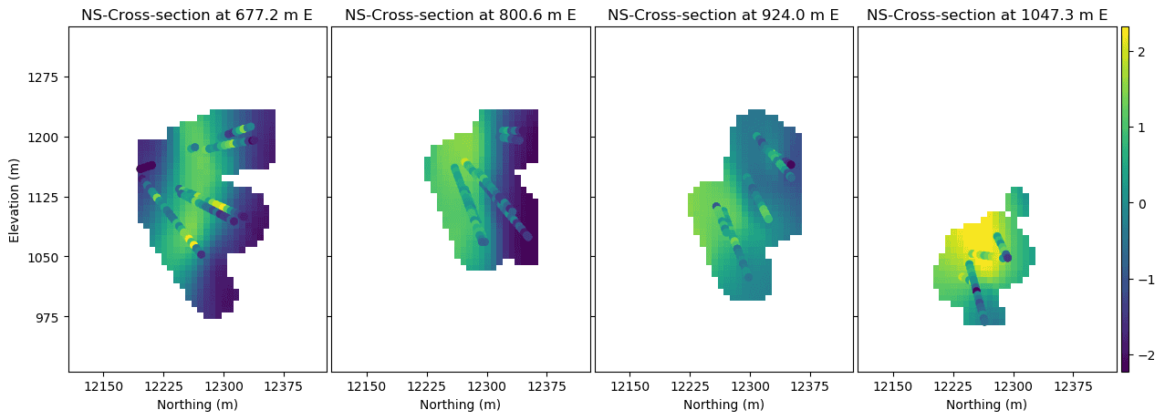
A numerical model of the deterministic trend is required. Kriging for the trend has not been successful because kriging aims for data reproduction and tends to the global mean at the margins of a domain. Geological variables are rarely amenable to a simple polynomial or functional trend shape. A weighted moving window average has proven effective. Some important implementation details to consider: (1) a length scale for the moving window specified for the primary direction of greatest continuity, (2) a Gaussian shape to the weighting function, (3) anisotropy in the kernel length scale somewhat less than that of the regionalized variable – often a square root of the anisotropy ratio to the maximum direction of continuity, (4) the weight to each data is the kernel weight multiplied by the declustering weight, and (5) a small background weight to all data of, say, one percent. The only free parameter is the length scale in the primary direction. Despite some worthwhile attempts to automate the calculation of this parameter it is set by experience and the visual appearance of the final model together with some metrics quantifying the relationship between the trend and residual. A value one third of the domain size may be reasonable. Once the trend is modeled, we must simulate with the trend. The following 3D trend model $m(\mathbf{u})$ comes from a kernel weighted moving window average of normal score transformed copper grades.

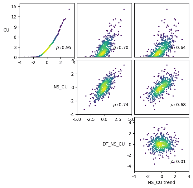
Creating a residual as $\{R(\mathbf{u})=Z(\mathbf{u})-m(\mathbf{u}), \mathbf{u}\; in\; A\}$ is not good practice. $Z$ and $m$ are related in complex ways causing $R$ and $m$ to be dependent. If $R$ is modeled independently then artifacts will be introduced in the $R+m$ back transformation. A stepwise conditional transform of the original variable conditional to the trend has proven effective. As shown in the figure below, this transform completely removes the dependence on the trend. Independent modeling proceeds and the reverse transform introduces the dependency between the original variable and the trend. The SCT considers a fitted Gaussian Mixture Model between the normal scores of the original variable and the normal scores of the trend. These normal score transforms are an intermediate step and are easily reversed. The workflow of trend modeling, data transformation, simulation and back transformation can be largely automated. There are, of course, validation steps that require the attention of a professional. The matrix of scatterplots below demonstrates the relationship between the original copper (CU) grades, normal score (NS) transformed grades, detrended normal score (DT_NS) grades, and trend model of the normal score data. Points are coloured by their kernel density.

The Resource Modeling Solutions Platform facilitates both trend modeling and modeling with a trend. This is a core requirement in modern probabilistic resource estimation and uncertainty assessment. The trend toward automation is also important.